Y = Observed Data, X = Completed Data 로 이해하며 읽을 것

Import

import numpy as np
import matplotlib.pyplot as plt

2. Self-Consistent Random Vectors

Suppose we want to represent or approximate the distribution of a random vector \(\bf{X}\) by a random vector \(\bf{Y}\) whose structure is less complex.

구조가 간단한(?) 확률벡터 Y로 확률벡터 X의 분포를 근사하거나 나타내려 한다고 하자.

One measure of how well \(\bf{Y}\) approximates \(\bf{X}\) is the mean squared error \(\cal{E}||\bf{X}-\bf{Y}||^2\).

Y로 X의 근사값을 잘 찾는 한 측정치는 평균제곱오차를 구하는 것이다.

In terms of mean squarred error, the approximation of \(\bf{X}\) by \(\bf{Y}\) can always be improved using \(\cal{E} [\bf{X}|\bf{Y}]\) since, for any function \(g\), \(\cal{E} ||\bf{X}-\cal{E} [\bf{X}|\bf{Y}]||^2 \le \cal{E} ||\bf{X}-g(\bf{Y})||^2\).

평균제곱오차에 관해 말하자면, Y에 의해 X의 근사치는 항상 Y 가 주어졌을때 X의 기대값으로 개선될 수 있는데, 어느 함수 g에 대해서나 위의 식이 성립한다.

\(\cal{E}\)\(||\bf{X}-\cal{E} [\bf{X}|\bf{Y}]||^2\) 이게 최솟값이라는 뜻

Taking \(g\) to be the identity gives \(\cal{E} || \bf{X} - \cal{E} [\bf{X}|\bf{Y}]||^2 \le \cal{E} ||\bf{X}-\bf{Y}||^2\).

함수 g에 Y를 주면, 위의 식이 된다.

E[X|Y] =Y일때 Y가 X에 대해 self-cosistent 하다고 했으니까 함수 g(Y) = Y라 한다면?

Thus the random vector \(Y\) is locally optimal for approximating \(\bf{X}\) if \(\bf{Y} = \cal{E} [\bf{X}|\bf{Y}]\), in which case we call \(Y\) self-consistent for \(\bf{X}\).

만일 Y가 Y가 주어졌을때 X의 기댓값과 같다면, 확률벡터 Y는 X에 근사하는데 있어 locally optimal 하다. 이때, Y를 X에 대해 self-consistent 하다고 부른다.

\(\cal{E}\)\(||\bf{X}-\cal{E} [\bf{X}|\bf{Y}]||^2\) 계산할때에 대해(locally) E(X|Y) = Y라면, 최적의 값(최소의 값, optimal)하다.

DEFINITION 2.1. For two jointly distributed random vectors \(\bf{X}\) and \(\bf{Y}\), we say that \(\bf{Y}\) is self-consistent for \(\bf{X}\) if \(\cal{E} (\bf{X}|\bf{Y}) = \bf{Y}\) almost surely.

두 결합 분포된 확률벡터 X와 Y에 대해 Y가 주어졌을때 X의 기댓값이 Y와 동일하다면 Y를 X에 대해 self-consistent 하다고 한다.

- 회귀에서 X를 추정하려 할 때, \(E(X|Y) = \hat{X}\)로 나타낼 수 있는데, \(E(X|Y) = \hat{X} = Y\)라면, Y는 X에 대해 self-consistent 하다.

1 \(\bf{Y} = \bf{X} + \epsilon\) \((\epsilon \sim i.i.d.)\)이라면, \(E(X|Y) = Y\) \(Y\)는 \(X\)에 대해 self-consistent 하다.

2 \(\bar{X} = \frac{1}{3}(X_1+X_2+X_3)\), \(\tilde{X} = \frac{1}{2}(X_2+X_3)\),

\(E(\bar{X}|\tilde{X}) = E(\frac{1}{3}X_1 + \frac{1}{3}\frac{1}{2}X_2 + \frac{1}{3}\frac{1}{2}X_3 | \tilde{X}) = E(\frac{1}{3}X_1|\tilde{X}) + E(\frac{1}{3}\frac{1}{2}X_2 + \frac{1}{3}\frac{1}{2}X_3 | \tilde{X})\)

self-consistent 되기 위한 조건

\(E(\frac{1}{3} X_1|\tilde{X})= E(\frac{1}{3} X_1)\) 이 \(\frac{1}{3} \tilde{X}\)이어야 한다.
\(E(X_1 | \tilde{X}) = E(X_1) = \tilde{X}\) 이어야 한다.
\(\mu = \tilde{X}\)이어야 한다.

\(\tilde{X}\)는 \(\bar{X}\)에 대해 self-consistent 하다.

We will assume implicitly that moments exist as required.

필요에 따라 이런 moment가 존재한다고 암묵적으로 가정할 것이다.

The notion of self-consistency is not vacuous, as the two extreme cases demonstrate.

두 극단적인 경우에서 나타나는 듯이, self-consistency는 모호한 개념이 아니다.

The random vector \(\bf{X}\) is self-consistent for \(\bf{X}\) and represents no loss of information.

확률 벡터 X는 X에 대해 self-consistent 하며, information의 손실이 전혀 없다.

\(\bf{Y} = \cal{E} [\bf{X}]\) is also self-consistent for \(\bf{X}\) and represents a total loss of information except for the location of the distribution.

Y=E(X)는 X에 대해 self-consistent 하며, 분포의 위치를 제외하고 information이 전체적으로 손실된다.

total loss of information은 만약 \(Y = \{Y_1,Y_2,... \}\) 있을때 값 신경 쓰지 않고 그냥 평균으로 사용할때이다.

Interesting self-consistent distributions range in between these two extremes.

이 두 극단적인 경우 사이에 self-consistent 분포들이 있다.

보류

loss of information 정의 정확히 짚기

1 \(\bf{X}\)는 information 손실이 없지만, \(\bf{Y}=E(X)\)는 \(\epsilon\)을 잃어서 information 손실이 생긴다.

Many relevant cases of self-consistency are obtained by taking conditional means over subsets of the sample space of \(\bf{X}\).

self-consistency의 많은 관련된 경우는 집합 𝐗의 표본 공간의 부분집합에 대한 조건부 평균을 취함으로써 구해진다.

Another simple example of self-consistency is the following:

또다른 self-consistency의 단순한 예제이다.

EXAMPLE 2.1. Partial sums. Let \(\{X_n\}\) denote a sequence of independent, mean-zero random variables, and let \(S_n = \sum^n_{i=1} X_i\).

부분합, x_n을 독립이고, 평균이 0인 확률 변수라고 할 때, x의 합을 Sn이라 두자.

Then \(\cal{E}\)\([S_{n+k}|S_n] = S_n + \cal{E}\)\([X_{n+1} + \dots + X_{n+k}|S_n] = S_n + \cal{E}\)\([X_{n+1} + \dots + X_{n+k}] = S_n\).

그러면 이 식이 성립함.

- 증명 \(\cal{E}\)\([S_{n+k}|S_n]=\)\(\cal{E}\)\([S_n + X_{n+1} + \dots + X_{n+k}|S_n]=\)\(\cal{E}\)\([X_{1} + \dots + X_n + X_{n+1} + \dots +X_{n+k}|S_n]=\)\(\cal{E}\)\([X_{n+1} + \dots + X_{n+k}] + S_n=S_n\)

Thus, \(S_n\) is self-consistent for \(S_{n+k}, k > 1\).

그려면 sn은 sn+k에 대해 self-consistent하다고 함.

The same property holds more generally if \(\{S_n\}_{n\ge1}\) represents a martingale process.

만일 저 식이 마틴게일 프로세스를 나타낸다면 동일한 특성이 유지된다.

Note

martingale process 의 특징

기댓값의 일정성
확률변수의 분포 고정

For a given \(\bf{X}\), a self-consistent approximation \(\bf{Y}\) can be generated by partitioning the sample space of \(\bf{X}\) and defining \(\bf{Y}\) as a random variable taking as values the conditional means, of subsets in the partition.

주어진 확률 변수 \(\bf{X}\)에 대한 self-consistent approximation \(\bf{Y}\)는 \(\bf{X}\)의 표본 공간을 분할하여 각 분할된 부분집합에 대한 조건부 평균을 값으로 가지는 랜덤 변수로 정의될 수 있다.

This is illustrated by our next example, in which the support of \(\bf{X}\) is partitioned into two half-planes.

다음 예제에서 확률 변수 \(\bf{X}\)의 support(모든 값?)가 두 개의 반 평면으로 나뉜다.(x1>=0,x1<0인듯?)

EXAMPLE 2.2. Two principal points. Let \(\bf{X} = (X_1, X_2)' \sim N_2(0, I_2)\). Note that \(\cal{E}\)\([X_1|X_1 \ge 0] = \sqrt{2/\pi}\). Let \(\bf{Y} = (-\sqrt{2/\pi}, 0)'\) if \(X_1 < 0\) and \(\bf{Y} = (\sqrt{2/\pi}, 0)'\) if \(X_1 \ge 0\). Then \(\bf{Y}\) is self-consistent for \(\bf{X}\).

\(\bf{Y} = \begin{cases}(-\sqrt{\frac{2}{\pi}}, 0)' & if X_1 < 0 \\ (\sqrt{\frac{2}{\pi}}, 0)' & if X_1 \ge 0 \end{cases}\)

\(\cal{E}\)\([X_1|X_1 \ge 0] = \bf{Y} = \sqrt{\frac{2}{\pi}}\)

Example 2.2 Uniform 버전

\(X_1 \sim U(0,1), X_2 \sim U(0,1)\) \((X_1,X_2)\)는 독립이라면, \(\cal{E}\)\([X_1|X_1 \ge 0.5] = 0.75\)

\(Y = \begin{cases}(0.25, 0)' & if X_1 < 0.5 \\ (0.75, 0)' & if X_1 \ge 0.5 \end{cases}\)

\(Y\)는 \(X_1\)이 0.5보다 클 때 0.75로, \(\cal{E}\)\([X_1|X_1 \ge 0.5]\)와 같다. 따라서 \(Y\)는 \(X\)에 대해 self-consistent하다.

See Section 6 for a definition of principal points, and see Figure 7 for a generalization of this example.

The preceding example illustrates the purpose of self-consistency quite well.

다음 예제는 self-consistency의 목적을 잘 나타낸다.

It is actually an application of our first lemma.

첫번째 lemma를 응용한 것이다.

Lemma 2.1. For a \(p\)-variate random vector \(\bf{X}\), suppose \(\mathcal{S} \subset \mathbb{R}^p\) is a measurable set such that \(\forall \bf{y} \in \mathcal{S}, \bf{y} = \cal{E}\)\([\bf{X} | \bf{X} \in \mathbb{D_y}]\), where \(\mathbb{D}_y\) is the domain of attraction of \(\bf{y}\), that is, \(\mathbb{D}_y = \{\bf{x} \in \mathbb{R}^p: ||\bf{x} - \bf{y}|| < ||\bf{x} - \bf{y}^*||, \forall \bf{y}^* \in \mathcal{S} \}\).

p변량 랜덤 벡터 X에 대해 p차원의 실수 집합의 부분 집합인 S가 측정 가능한 집합이고, 모든 y가 S에 속할때, y는 y에 수렴하는 도메인 Dy에 X가 속하는 조건에서 X의 기댓값과 같다.

Dy(the domain of attraction) = x는 p차원의 실수 집합(R^p)에 속하는 값이고, p차원의 실수 집합(R^p)의 부분 집합(S)에 속하는 모든 y * 에 대해 x,y 의 거리가 x,y * 의 거리보다 짧은 값들의 집합

Defne \(\bf{Y} = \bf{y}\) if \(\bf{X} \in \mathbb{D}_y\): Then \(\bf{Y}\) is self-consistent for \(\bf{X}\).

X가 y의 domain of attration에 속한다면, Y=y라고 정의하며, Y는 X에 대해 self-consistent 하다.

Proof. \(\cal{E}\)\([\bf{X} | \bf{Y}=\bf{y}] =\)\(\cal{E}\)\([\bf{X}|\bf{X} \in \mathbb{D}_y] = \bf{y}\).

In Example 2.2, \(\cal{S}\) consists of only two points, and the associated domains of attraction are the half-planes given by \(x_1 < 0\) and \(x_1 > 0\).

예제 2.2에서 S는 두 점으로 구성되어 있고, associated domain of attraction은 x_1<0이거나 x_1>0인 half-plane이다.

예제 2.2에서 lemma2.1 찾기

\(p = 2\), p 변량 확률 벡터 \(\bf{X} = (X_1, X_2)' \sim N_2(0, I_2)\) 에 대해
p차원 실수 집합의 부분 집합인 \(S = \{ (-\sqrt{2/\pi}, 0)', (\sqrt{2/\pi}, 0)' \}\)가 모든 y가 S에 속한다는 조건 아래 측정 가능한 집합일때,
\(y = \cal{E}\)\([\bf{X} | \bf{X} \in \mathbb{D_y}]\) 이다.
The domain of attraction은 \(X_1 \ge 0\), \(X_1 < 0\)인 half-plane

- \(X\)가 \(\mathbb{D}_y\)에 속한다면, \(\cal{E}\)\([X_1|X_1 \ge 0] = \sqrt{2/\pi}\) 여기서 \(X_1 \ge 0\) 조건이 \(X\in \mathbb{D}_y\)와 동등한 개념으로 보인다.

The following three lemmas give elementary properties of self-consistent random vectors.

다음 세 개의 lemma는 self-consistent한 랜덤 벡터의 기본적인 특성을 제시한다.

Lemma 2.2. If \(\bf{Y}\) is self-consistent for \(\bf{X}\), then \(\cal{E}\) \([\bf{Y}]=\)\(\cal{E}\)\([\bf{X}]\).

Y가 X에 대해 self-consistent하다면, Y의 기댓값은 X의 기댓값과 같다.

Proof. The lemma follows from \(\cal{E}\)\([\cal{E}\)\([\bf{X}|\bf{Y}]]=\)\(\cal{E}\)\([\bf{X}]\)

We now introduce notation for the mean squared error (MSE) of a random vector \(\bf{Y}\) for \(\bf{X}\),

\(MSE(\bf{Y};\bf{X})=\cal{E}\)\(||\bf{X}-\bf{Y}||^2\)

The next lemma relates the MSE of a selfconsistent Y for X in terms of their respective covariance matrices.

다음 lemma는 X에 대해 self-consistent한 Y의 MSE와 관련있는데, 이를 공분산 행렬로 각각 나타낼 것이다.

Here, \(\Psi_\bf{X}\) and \(\Psi_\bf{Y}\) denote the covariance matrices of \(\bf{X}\) and \(\bf{Y}\), respectively.

공분산 X,Y를 쓰는 법

\(\Psi_{X} = \text{Cov}(X) = \begin{bmatrix} \text{Cov}(X_1, X_1) & \text{Cov}(X_1, X_2) & \cdots & \text{Cov}(X_1, X_p) \\ \text{Cov}(X_2, X_1) & \text{Cov}(X_2, X_2) & \cdots & \text{Cov}(X_2, X_p) \\ \vdots & \vdots & \ddots & \vdots \\ \text{Cov}(X_p, X_1) & \text{Cov}(X_p, X_2) & \cdots & \text{Cov}(X_p, X_p) \\ \end{bmatrix}\)

\(\Psi_{Y} = \text{Cov}(Y) = \begin{bmatrix} \text{Cov}(Y_1, Y_1) & \text{Cov}(Y_1, Y_2) & \cdots & \text{Cov}(Y_1, Y_p) \\ \text{Cov}(Y_2, Y_1) & \text{Cov}(Y_2, Y_2) & \cdots & \text{Cov}(Y_2, Y_p) \\ \vdots & \vdots & \ddots & \vdots \\ \text{Cov}(Y_p, Y_1) & \text{Cov}(Y_p, Y_2) & \cdots & \text{Cov}(Y_p, Y_p) \\ \end{bmatrix}\)

Lemma 2.3. If \(\bf{Y}\) is self-consistent for \(\bf{X}\), then the following hold: (i) \(\Psi_\bf{X}\) \(\ge \Psi_\bf{Y}\), that is, \(\Psi_{\bf{X}} - \Psi_{\bf{Y}}\) is positive semidenite; (ii) \(MSE(\bf{Y};\bf{X})= tr(\Psi_{\bf{X}}) - tr(\Psi_\bf{Y})\):¹

¹ 결국 \(tr(\Psi_{\bf{X}}) - tr(\Psi_\bf{Y})\)를 계산하면 분산이 같은 값의 부분은 0이 되고, 값이 다른 부분만 남겠지

Y가 X에 대해 self-consistent하다면, X의 공분산행렬은 Y의 공분산행렬보다 크다. MSE는 X의 공분상행렬의 대각행렬에서 Y의 공분산 행렬의 대각 행렬을 뺀 것과 같다.(X의 분산 - Y의 분산 과 같다.)

Important

예를 들어 x,y가 아래와 같이 있을때,(\(E(x)=0, x_1\)이 결측이라 평균인 0으로 대체)

\(x = {0.2,-0.3,0.5}, y = {0,-0.3,0.5}\) (단, x는 completed data, y는 observed data라고 이해할때)

평균으로 바꾼 y가 x의 분산보다 작다. 변동이 작아져서

\(\text{tr}(\Psi_{X}) = \text{Cov}(X_1, X_1) + \text{Cov}(X_2, X_2) + \cdots + \text{Cov}(X_p, X_p) = Var(X)\)

\(\text{tr}(\Psi_{Y}) = \text{Cov}(Y_1, Y_1) + \text{Cov}(Y_2, Y_2) + \cdots + \text{Cov}(Y_p, Y_p) = Var(Y)\)

See the Appendix for a proof.

appendix Proof of Lemma 2.3. Without loss of generality assume \(\cal{E}\)\([\bf{X}] = 0\). For part (i), by self-consistency of \(\bf{Y}\) for \(\bf{X}\) and using the conditional variance formula \(Cov[\bf{X}] = Cov[\cal{E}\)\([\bf{X}|\bf{Y}]]+ \cal{E}\)\([Cov[\bf{X}|\bf{Y}]]\), we have \(Cov[\bf{X}] =\)\(Cov[\bf{Y}] + \cal{E}\)\([Cov[\bf{X}|\bf{Y}]]\). But \(Cov[\bf{X}|\bf{Y}]\) is positive semidefinite almost surely, and hence (i) follows. For part (ii) we have

\(\cal{E}\)\(||\bf{X}-\bf{Y}||^2 =\) \(\cal{E}\)\([\bf{X}'\bf{X}] -\) \(2\cal{E}\)\([\bf{Y'X}] +\) \(\cal{E}\)\([\bf{Y'Y}]\)

\(= tr(\Psi_\bf{X})-\) \(2\cal{E}[\cal{E}\)\([\bf{Y'X|Y}]]+\) \(tr(\Psi_\bf{Y})\).

\(= tr(\Psi_\bf{X})-\) \(2\cal{E}\)\([\bf{Y'}\cal{E}\)\([\bf{X|Y}]]+\) \(tr(\Psi_\bf{Y})\).

\(= tr(\Psi_\bf{X})-\) \(2\cal{E}\)\([\bf{Y'Y}]+\) \(tr(\Psi_\bf{Y})\).

\(= tr(\Psi_\bf{X})-\)\(tr(\Psi_\bf{Y})\).

다시 써보기

\(E||X - Y||^2 = E(XX' - X'Y - Y'X + YY')\)

\(= E(X^2 - 2Y'X + Y^2)\)

\(= tr(\Psi_X) - 2 E(E(Y'X|Y)) + tr(\Psi_Y)\)

\(= tr(\Psi_X) - 2 E(Y'E(X|Y)) + tr(\Psi_Y)\)

\(= tr(\Psi_X) - 2 E(Y'Y) + tr(\Psi_Y)\)

\(= tr(\Psi_X) - 2tr(\Psi_Y) + tr(\Psi_Y)\)

\(= tr(\Psi_X) - tr(\Psi_Y)\)

- \(E(Y'X) = E(E(Y'X|Y))\) \(\to\) 전체 기댓값의 법칙

전체 기댓값의 법칙 증명(이산확률변수에서)

\(E(E(X|Y)) = E(X)\) 일때,

\(E(E(X|Y))\)

\(= \sum_{y \in Y} p(y)E(X|Y)\)

\(= \sum_{y \in Y} p(y) \sum_{x \in X} p(x|y) x\)

\(= \sum_{y \in Y} \sum_{x \in X} p(y) p(x|y) x\)

\(= \sum_{y \in Y} \sum_{x \in X} p(x,y) x\)

\(= \sum_{x \in X} p(x) x = E(X)\)

It follows from Lemma 2.3 that \(Cov[\bf{Y}] =\)\(Cov[\bf{X}]\) exactly if \(Cov[\bf{X}|\bf{Y}] = 0\) a.s., that is, if \(\bf{Y} = \bf{X}\) a.s.

lemma 2.3의 \(Cov[\bf{X}] = Cov[\cal{E}\)\([\bf{X}|\bf{Y}]]+ \cal{E}\)\([Cov[\bf{X}|\bf{Y}]]\) 여기서 \(Cov[\bf{X}|\bf{Y}]\)이 0이 된다면,

\(Cov[\bf{X}] = Cov[\cal{E}\)\([\bf{X}|\bf{Y}]]\), 근데 Y가 X에 대해 self-consistent할 때 \(\cal{E}\)\([\bf{X}|\bf{Y}] = Y\),

따라서 \(Cov[{X}] = Cov[Y]\)

For one-dimensional random variables \(\bf{X}\) and \(\bf{Y}\), if \(\bf{Y}\) is self-consistent for \(\bf{X}\), then \(var[\bf{Y}]\) \(\le var[\bf{X}]\), with equality exactly if \(\bf{Y}\)\(=\bf{X}\) a.s.

There is a similarity between the two preceding lemmas and the Rao{Blackwell theorem (Casella and Berger, 1990, page 316), which in a simplied version states the following.

If \(\bf{X}\) is an unbiased estimator of a parameter \(\theta\), and if \(\bf{Y}\) is a sufcient statistic for \(\theta\), then \(\cal{E}\)\([\bf{X}|\bf{Y}]\) is an unbiased estimator of \(\theta\), and \(var[\cal{E}\)\([\bf{X}|\bf{Y}]\)\(\le var[\bf{X}]\). If \(\cal{E}\)\([\bf{X}|\bf{Y}\)\(] = \bf{Y}\), then Lemma 2.2 gives \(\cal{E}\)\([\bf{Y}\)\(] = \cal{E}\)\([\bf{X}]\), and part (i) of Lemma 2.3 gives \(var[\bf{Y}]\le var[\bf{X}]\).

1차원 확률 벡터 X,Y에 대해 Y가 X에 대해 self-consistent하다면, Y의 분산은 X의 분산보다 작거나 같다.(단, Y=X로 정확히 일치할때만??)

만일 X가 세타에 대한 비편향 추정량이고(\(E(X)=\theta\), That is,\(X=\hat{\theta}\),X의 기댓값이 세타와 같다면),
만일 Y가 세타에 대한 충분 통계량이라면(Y가 세타에 대한 충분한 정보가 있어서 세타를 효율적으로 표현할 수 있다면)

Y가 주어졌을때 X의 기댓값은 세타에 대한 비편향 추정량이고(Y가 주어졌을때 X의 기댓값이 세타와 같고),
Y가 주어졌을때 X의 기댓값의 분산은 X의 분산보다 작거나 같다.

- 만일 Y가 주어졌을때 X의 기댓값이 Y라면(Y가 X에 대해 self-consistent 하다면)

lemma 2.2에서 X의 기댓값이 Y의 기댓값과 같다고 할 수 있고,
lemma 2.3에서 Y의 분산이 X의 분산보다 작거나 같다고 할 수 있다.

The next lemma demonstrates a dimensionality reducing property of self-consistent random variables.

다음 lemma는 self-consistent 확률 변수의 차원적으로 감소하는 특징에 대해 설명한다.

Here, \(\cal{S}\)\((\bf{Y})\) denotes the support of \(\bf{Y}\).

S(Y)는 Y의 support를 의미

Y의 support = Y의 집합?

Lemma 2.4. Suppose \(\bf{Y}\) is self-consistent for a \(p\)-variate random vector \(\bf{X}\) with \(\cal{E}\)\([\bf{X}] = 0\), and \(\cal{S}\)\((\bf{Y})\) is contained in a linear subspace spanned by \(q\) orthonormal column vectors in the \(p \times q\) matrix A.

p 변량 확률 벡터 X에 대해 X의 기댓값이 0일때 Y가 이 X에 대해 self-consistent 하다고 가정하면, S(Y) 는 p행 q열인 행렬 A에서 q열이 직교한 열벡터애 의해 생성된 선형 부분 공간에 포함된다.

Note

\(\to\) q열이 직교한다 \(\to\) q열끼리 곱하면 0이 된다. \(\to\) q열은 서로 독립이다.

선형 공간 linear space = 벡터 공간 vector space

Let \(P = AA'\) denote the associated projection matrix.

Then \(\bf{Y}\) and \(\bf{A'Y}\) are self-consistent for \(\bf{PX}\) and \(\bf{A'X}\), respectively.

Projection Matrix 투영행렬

투영행렬의 정의

어떤 벡터를 다른 어떤 공간으로 투영시키는 것

투영행렬의 특징

\(P =P^\top\) 대칭이고,
\(P^2 = P\) 두 번 투영시켜도 결과는 그대로다.
ex) 단위행렬 \(\begin{bmatrix} 1 & 0 \\ 0 & 1 \end{bmatrix}\)
ex) 0행렬 \(\begin{bmatrix} 0 & 0 \\ 0 & 0 \end{bmatrix}\)
ex) 2차원을 1차원으로 축소하는 \(P=\begin{bmatrix} 1 \\ 0 \end{bmatrix}\) \(\to\) 하나의 축에 투영하는 법

- PCA로 이해해보자..\(X = n \times d\) matrix , \(P = d \times k\) matrix

\(X\)의 공분산 행렬 C를 이용한 고유값 분해 \(C = V \Lambda V^T\)
차원 축소하면 \(Y = XP\)

- 특이값 분해로 이해해보자.. \(A = U \sum V^T\)

여기서 U,V는 직교 행렬으로 \(I = U^T U\), \(I = V^V V\)을 만족
- \(U = m \times m\), \(\sum=m \times n\), \(V = n \times n\)
- U, V는 P 투영 행랼?

See the Appendix for a proof.

appendix Proof of Lemma 2.4. Since \(\bf{Y}\) is self-consistent for \(\bf{X}\), \(\cal{E}\)\([\bf{PX|Y}] = \bf{P}\cal{E}\)\([\bf{X|Y}] = \bf{PY} = \bf{Y}\) a.s.

For a given \(\bf{y} \in \mathbb{R}^p\), let \(\bf{w = A^{'}_{1} y}\).

Then \(\{ \bf{Y} = \bf{y} \} = \{A^{'}_{1} Y = w\}\).

Multiplying both sides of the equation \(\cal{E}\)\([\bf{X|Y = y] = y}\) on the left by \(A^{'}_{1}\) gives \(\cal{E}\)\([\bf{A^{'}_{1} X|A^{'}_{1} Y} = w] = w\).

Lemma 2.4 means that the marginal distribution of a self-consistent \(\bf{Y}\) in the linear subspace spanned by its support is self-consistent for the marginal distribution of \(\bf{X}\) in the same subspace.

lemma 2.4가 의미하는 것은 그 support에 의해 생성된 선형 부분 공간에서 self-consistent한 Y의 주변 분포는 같은 부분공간에서 X의 주변 분포에 대해 self-consistent한 것이다.

For example, a self-consistent distribution for \(\bf{X}\) whose support consists of a circle (see Section 6) is determined by the bivariate marginal distribution of \(\bf{X}\) in the subspace containing the circle.

예를 들어, support가 원으로 구성된 X에 대해 self-consistent한 분포는 원을 포함한 부분 공간에서 X의 이변량 주변 분포에 의해 결정된다.

In Example 2.2, the linear subspace spanned by the support of \(\bf{Y}\) is the \(x_1\)-axis, the marginal distribution of \(\bf{X}\) in this subspace is standard normal, and the random variable \(\bf{Y}_1 = sgn(\bf{X}_1)\sqrt{2/\pi}\) is self-consistent for \(\bf{X}_1\).

예제 2.2에서 Y의 support에 의해 생성된 선형 부분 공간은 x1축이고, 부분 공간에서 X의 주변 분포는 표준정규분포이고, X1의 값에 따라 바뀌는 확률변수 Y1은 X1에 대해 self-consistent하다.

Sign Function 부호 함수

기호는 sgn로 표현, 수의 부호 판별하는 함수

example 2.2처럼 y를 x를 기준으로 나눠서 함수 쓸 때 사용할 수 있음.

# x 값의 범위 설정
x = np.linspace(-5, 5, 100)

# 부호 함수 정의
def sgn(x):
    if x > 0 :
        y = 1
    elif x < 0 :
        y = -1
    elif x == 0 :
        y = 0
    return y

# 그래프 그리기
plt.plot(x, [sgn(x[i]) for i in range(len(x))], label='sgn(x)')
plt.xlabel('x')
plt.ylabel('sgn(x)')
plt.ylim(-1.5,1.5)
plt.xlim(-4,4)
plt.title('Sign Function')
plt.grid(False)
plt.legend()
plt.show()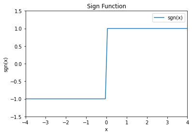

We conclude this section with a general method of finding self-consistent random variables.

Lemma 2.5. Let \(\bf{X}\) and \(\bf{Y}\) denote two jointly distributed random vectors, not necessarily of the same dimension.

Then \(\cal{E}\)\([\bf{X}|\bf{Y}]\) is self-consistent for \(\bf{X}\).

Proof. Let \(\bf{Z} = \cal{E}\)\([\bf{X}|\bf{Y}]\). Then \(\cal{E}\)\([\bf{X}|\bf{Z}] = \cal{E}[\cal{E}\)\([\bf{X}|\bf{Y}]|\bf{Z}] = \cal{E}[\bf{Z}|\bf{Z}] =\bf{Z}\)

In particular, setting \(\bf{Y} = \bf{X}\) in Lemma 2.5 gives again self-consistency of \(\bf{X}\) for itself.

If \(\bf{Y}\) is independent of \(\bf{X}\), then it follows that \(\cal{E}\)\([\bf{X}]\) is self-consistent for \(\bf{X}\).

X와 Y가 결합 확률 벡터일때, Y를 고려한 X의 기댓값은 X에 대해 self-consistent 하며, 특히 Y가 X와 같을 때 lemma 2.5에 나온 E(X|Y)는 X에 대해 self-consistent하다는 것에 의해 X는 자기 자신에 대해 self-consistency하다는 것을 얻을 수 있다.

만약 Y가 X에 대해 독립이라면 X의 기댓값은 X에 대해 self-consistent하다.